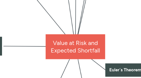
1. Marginal, Incremental, and Component Measures
1.1. A portfolio is composed of a number of subportolios could correspond to asset classes.
1.2. Analysts calculate measures of the contribution of each sub-portfolio tO VaR or ES
1.3. Supposing that the amount invested in a portfolio is xi. The marginal value at risk for the ith subportfolio is the sensitivity of VaR to the amount invested in the ith subportfolio.
1.3.1. Formula: o/VaR/0/xi
1.4. The component value at risk for the ith subportfolio is:
1.4.1. Ci= (o/VaR/0/xi)xi
1.5. This can be approximated as
1.5.1. (/_\VaR//_\xi)xi
2. Aggregating VaRs and ESs
2.1. This works in business to calculate the total VaR.
2.1.1. VaRtotal = Square rooth of (E)i(E)j VaRi VaRj Pij
2.2. VaRi = VaR for the ith segment
2.3. Pij= Correlation between losses from segment i and segment j.
2.4. This is true when losses or gains have zero-mean normal distributions and provides a good approximation in many other situations.
3. Expected Shortfall:
3.1. The expected shortfall is another measure . That can calculate the expected loss.
3.2. Expected shortfall has two parameters. T(The time horizon) and X(The confidence level).
3.3. To calculate the Expected Shortfall you need to calculate first the VaR.
3.4. Recognizes the diversification.
3.5. Is more difficult to understand than VaR.
4. Coherent Risk Measures
4.1. Properties that a risk measure should have:
4.1.1. Monotonicity: If a portfolio produces less than other portfolio, the risk measure should be greater.
4.1.2. Translation Invariance: If an amount of cash is added to a portfolio, risk should go down.
4.1.3. Homogeneity: Risk measure multiplied when changing size of portfolio.
4.1.4. Subadditivity: The risk measure for two portfolios after merged should be no greater than the sum of their risk measures before merged.
4.1.5. The three conditions satisfies the measure of VaR. Although it the fourth condition, does nos satisfies because if we add one portfolio the risk can stay the same or decrease.
5. Definition of VaR:
5.1. Analysis or attempt to provide a single number that summarizes the total risk of a whole portfolio. So is making sure that "X%" certain that we will not lose more than "V" money in time "T".
5.2. V: VaR= Value at Risk of the Portfolio.
5.3. X: Confidence Level
5.4. T: Time
6. Choice of Parameters for VaR and ES
6.1. User must choose two parameters: T and X
6.2. This is useful to consider the consequences of the assumption at this stage.
6.3. Loss in the portfolio value has a mean of u and sd of o-
6.3.1. VaR = u + o-N^-1 (X)
6.3.2. NORMSINV In Excel
6.4. When loss is assumed to be normally distributed with mean u and sd, ES with a confidence level of X is given by:
6.4.1. ES= u+o-(e^-Y^2/2 / 2PI^1/2 (1-X)
6.5. The application, when market risks are being considered, is by calculation VaR or ES for a time horizon, the assumption is:
6.5.1. T-day VaR = 1-DAY VaR x rooth of T
6.5.2. T-day ES = 1- day ES = 1- day ES x rooth of T
6.6. Impact of Autocorrelation: The value of a portfolio from one day to the next are not always totally independent.
6.6.1. o-+o^2+2po-^2=2(1+p)o-^2
6.7. Confidence Level
6.7.1. Depends in a number of factors. Contemplates credit rating, period, type of firm.
7. Euler´s Theorem
7.1. When a risk measure for a whole portfolio is allocated to subportfolios.
7.2. V= RISK MEASURE FOR A PORTFOLIO and Xi= is a measure of the size of the ith subportfolio (1<i<M)
7.3. V= M(E)i=1(o/V/o/xi)xi
7.4. When the risk measure is VaR, Eulers theorem gives.
7.4.1. VaR=M(E)i=1Ci
7.5. When the risk measure is ES, Eulers theorem similarly shows that the total ES is the sum of the component ESs:
7.5.1. ES=(M(E)i=1)(o/ES/o/xi)xi
8. Back-Testing
8.1. This a reality check for risk measure. It is a test of how well the current procedure for calculating the measure would have worked in the past
8.2. It can be calculated for VaR and ES.
8.3. Involves looking at how often the loss in a day would have exceeded.
8.4. One issue of a one-day VaR to consider changes made in the portfolio during a day.
8.5. The prob of an exception on any given day is p or greater than p.
8.5.1. (n(E)k=m)(n!/k!(n-k)!)((p^k)(1-p)^n-k))
8.6. When number of exceptions,m, is lower than the expected number of exceptions.
8.6.1. (n(E)k=o)(n!/k!(n-k)!)((p^k)(1-p)^n-k))
