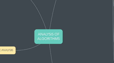
1. WORST AND BEST CASE ANALYSIS
1.1. Algorithms with a running time dependant on the input data size and content
1.2. End of execution depends on conditions
1.3. Worst and Best case analysis
1.3.1. Worse Case: usually higher growth functions
1.3.2. Best Case: lower growth functions, or usually a growth function whereby T(N) = 1
2. ASYMPTOTIC ANALYSIS
2.1. WHAT IS ASYMPTOTIC ANALYSIS?
2.1.1. Analyzing algorithms when the input data is large
2.1.1.1. OMEGA NOTATION
2.1.1.1.1. proposed to analyze functions in the area of math
2.1.1.1.2. Invention: 1914, Godfrey Hardy and Joan Littlewood
2.1.1.1.3. Defines a set of functions that act as a lower bound of T(N) T(N) is omega g(N)) if: c*g(N) <= T(N) for all N >=n0; where c,n are positive constants
2.1.1.2. BIG-O NOTATION
2.1.1.2.1. used to describe the behaviour of a function when its argument tends to infinity
2.1.1.2.2. Invention: 1894, Paul Bachmann, well before modern computer architecture
2.1.1.2.3. Defines a set of functions that act as an upper bound of T(N) T(N) is O (g(N)) if: c*g(N) >= T(N) for all N >=n0; where c,n are positive constants
2.1.1.3. THETA NOTATION
2.1.1.3.1. was proposed especially for algorithm analysis in the field of computer science
2.1.1.3.2. Invention: 1970
2.1.1.3.3. Theta notation finds a single function that acts simultaneously as an upper or lower bound for our running time function or memory space function T(N) is theta (g(N)) if: c*g(N) >= T(N) for all N >=n0; where c,n are positive constants c*g(N) <= T(N) for all N >=n0; where c,n are positive constants
2.1.2. All 3 notations study the behaviour of a function where the argument tends to infinity
3. INTRO TO ANALYSIS OF ALGORITHMS
3.1. WHAT IS ANALYSIS OF ALGORITHMS?
3.1.1. Algorithms can be analysed with respect to 3 aspects; CORRECTNESS; EASE OF UNDERSTANDING and COMPUTATIONAL RESOURCE CONSUMPTION
3.1.1.1. CORRECTNESS
3.1.1.1.1. Performing a specific task according to a given specification
3.1.1.2. EASE OF UNDERSTANDING
3.1.1.2.1. Functions which implement specific algorithms are usually part of larger programs which are maintained and updated by different people at various times
3.1.1.2.2. Future development teams should be able to understand the meaning behind the algorithms implemented, and what the author was trying to execute using the algorithms
3.1.1.3. COMPUTATIONAL RESOURCE CONSUMPTION
3.1.1.3.1. Algorithms use processing and memory resources when executed (and sometimes bandwidth)
3.1.1.3.2. The lower the resources used, the better the algorithm in terms of analysis
3.1.1.3.3. Important Questions for Analysing Algorithms
3.2. MEASURING/ESTIMATION OF TIME AND SPACE REQUIREMENTS
3.2.1. 2 APPROACHES
3.2.1.1. Empirical Approach: Implementing algorithm in a particular programming language executed in a specific machine and then somehow measuring its execution time and memory requirements.
3.2.1.1.1. Pros: - Real / Exact results - No need for calculations
3.2.1.1.2. Cons: - Machine-Dependent Results - Implementation Effort
3.2.1.2. Theoretical Approach: Making reasonable assumptions about no. of CPU operations the algorithm is going to perform, counting new variables and calculating memory space
3.2.1.2.1. Pros: - Universal Results - No Implementation Effot
3.2.1.2.2. Cons: - Approximate results - Calculations Effort
3.2.1.2.3. Working on this approach: 1. Learning about the machine model 2. Knowing the assumptions 3. Do the calculations
3.3. RAM MODEL
3.3.1. Random Access Machine model
3.3.1.1. Used to analyze the running time and memory requirements of the algorithms
3.3.1.2. ASSUMPTIONS
3.3.1.2.1. RUNNING TIME
3.3.1.2.2. MEMORY SPACE
3.4. COUNTING UP OF TIME AND SPACE UNITS
3.4.1. using pseudo code of algorithms
3.4.1.1. SIMPLE ALGORITHM (w/o loops)
3.4.1.2. COMPLEX ALGORITHM (with for loops)
4. GROWTH OF FUNCTIONS
4.1. Taking so much time and effort in counting up every single time unit is not necessary if we just want to compare differnet algorithms and select the fastest one
4.1.1. Applies to both running times and memory requirements
4.1.1.1. Growth functions aid with
4.1.1.1.1. Comparing Algorithms efficiently
4.1.1.1.2. easing the process of calculating the running time manually which is very tedious and error prone
4.1.1.2. We focus on the big values of N
4.1.1.3. Coefficients and lower-order terms are NOT important when defining growth
4.1.1.3.1. Typical Growth Functions: (fastest to slowest) 1 logN N NlogN N^2 N^3 2^N N!
4.2. Calculating the growth of the running time of an algorithm without counting every single time unit
4.2.1. use a GENERIC CONSTANT to refer to the time units taken by simple operations
4.3. Faster Computer VS Faster Algorithm
4.3.1. Investing time in a faster algorithm is ALWAYS better than investing money on a faster computer
4.3.2. Very big instances are only solved with growth functions N or NlogN, or slower
4.3.3. Quadratic and higher growth functions are only useful for small instances
