

1. Getting ready
1.1. introducing Python's Pysal
1.1.1. using graph to represent matrices
1.1.1.1. focal
1.1.1.2. focal's neighbor(s)
1.1.1.3. edges
1.2. maps
1.2.1. USA states
1.2.1.1. "Four Corners" helps understand most concepts
1.2.1.1.1. we will subset usa_maps
1.2.2. Peru "districts"
1.2.2.1. maps with social data
1.2.3. projected CRS
2. Neighborhood
2.1. matrix representation
2.1.1. distance matrix
2.1.1.1. sub usa
2.1.2. neighborhood Matrix
2.1.2.1. binary matrix
2.1.2.1.1. contiguity
2.1.2.1.2. proximity
2.1.2.2. continuous matrix
2.1.2.2.1. contiguity
2.1.2.2.2. proximity
3. Neighborhood as WEIGHTS
3.1. all previous matrices
3.1.1. the sum by row
3.1.1.1. unnormalized weights
3.1.1.1.1. The sum of the rows does NOT equal 1.
3.2. normalized weights
3.2.1. transforming values per row
3.2.1.1. a row adds to 1 (ONE)
3.2.1.1.1. from
3.2.1.1.2. to
4. the spatial lag: **HOW ARE MY NEIGHBORS DOING...?**
4.1. How am I doing?
4.1.1. choropleth
4.2. How is my situation related to my neighborhood?
4.2.1. uses the normalized matrix
4.2.1.1. to weight social data values of neighbors
4.2.2. Each **lag** is the average of the neighbor values (the social data) weighted by the normalized row values of the adjacency matrix.
4.2.2.1. here, my education level (X) follows a direct relationship with my neighbors level (Y)
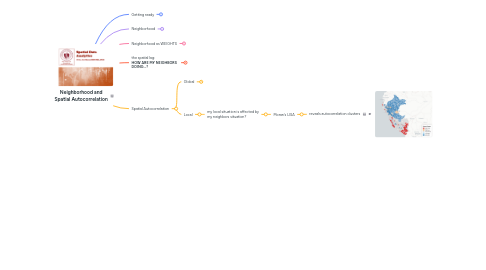
5. Spatial Autocorrelation
5.1. Global
5.1.1. my variable values is affected by my neighbors' variable values?
5.1.1.1. Moran's I
5.1.1.1.1. coefficient (similar to Pearson's R) measuring the relationship between a variable and its lag
5.2. Local
5.2.1. my local situation is affected by my neighbors situation?
5.2.1.1. Moran's LISA
5.2.1.1.1. reveals autocorrelation clusters