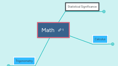
1. Trigonometry
1.1. The Unit Circle
1.1.1. Trigonometry, despite the many associated functions, and the seemingly complex equations, is essentially a set of functions that model the rate of change of a circle.
1.1.1.1. This is displayed by a graphed circle with a radius equal to one, centered over the origin on the coordinate plane. The circle can be measured in either degrees, as is common for most angle measurements, or in radians.
1.1.1.1.1. Radians are a measurement that works in terms of pi. 90 degrees is equivalent to half pi, 180 to pi, 270 to three halves pi, and 360 to two pi.
1.1.1.1.2. Trigonometric functions in their parent function form (without modifications to position, amplitude, or frequency) model the rate of change of the unit circle.
1.2. Trigonometric Calculus
1.2.1. Derivative and rate of change can also be used to model the trigonometric functions.
1.2.1.1. The derivative of the sine function is the cosine function.
1.2.1.2. The derivative of the cosine function is the negative sine function.
1.2.1.3. While easy to remember once calculated, the actual math is quite long winded and complicated. But it essentially uses proven trigonometric identities to change the form of the equation so that it fits the derivative formula, and so that the variable h is removed.
1.2.1.3.1. One example of these identities is as follows: sin^2 (x)+ cos^2 (x) = 1
1.3. Applications
1.3.1. Trigonometric functions can be used to model various functions in the natural world.
1.3.1.1. Radioactivity
1.3.1.1.1. From using parametric functions (a function dependent on a parameter) to accounting for change over time, to applying derivatives to the trigonometric functions to calculate the distance traveled, velocity, and acceleration of the electromagnetic waves (gamma rays), calculus and trigonometry enable radiation to be used with precision, allowing safe uses for otherwise dangerous (through unhealthy levels of exposure) radioactivity.
1.3.1.2. Modeling Temperature
1.3.1.2.1. While less dangerous than exposure to radioactivity, temperature variations throughout the year are equally applicable to trigonometric models. Average temperature fluctuations throughout the year mimic the patterns of trigonometric functions, allowing scientists and analysts to predict temperature trends based on the trigonometric functions and their derivatives.
2. Statistical Significance
2.1. Hypothesis testing
2.1.1. See T-testing; the relevant parts of the processes are similar.
2.2. T-testing
2.2.1. Confidence Intervals
2.2.1.1. P-values
2.2.1.1.1. Choosing the confidence interval or the associated p-value is a judgement.
3. Calculus
3.1. Derivatives
3.1.1. Rate of Change
3.1.1.1. Rate of Change in math is essentially delta y/delta x or the change in y divided by the change in x. This is equivalent to the slope formula for linear functions.
3.1.1.1.1. An additional formula is necessary for finding the rate of change for non linear functions, this formula finds the derivative of a function.
3.1.2. A derivative is essentially a function that describes the rate of change of another function - this is needed because not all functions can have their rate of change described numerically.
3.1.2.1. The derivative of a function is taken by finding the slope for a given point on the function. It then uses limits to achieve a a slope that is as close as possible to the behavior of the function.
3.1.2.2. In other words, the derivative determines the slope at any possible point on the function. It uses the following equation:
3.1.2.2.1. With the limit h -> 0, (f(x+h) -f(x))/h
3.1.3. Derivatives have many applications outside of the study of mathematics. One of these applications is in calculation made in physics.
3.1.3.1. The formulas representing the scalar and vector quantities of distance, velocity, acceleration can be used to find one another.
3.1.3.1.1. The derivative of distance is velocity, the derivative of velocity is acceleration (for constant acceleration). Essentially the different quantities describe the rate of change of each other.
3.2. Intergrals
3.2.1. Measurement of the area under the curve.
3.2.1.1. Riemann Sums
3.2.1.1.1. Riemann sums are a type of technique that allow the approximate area under the function to be calculated.
3.2.2. Integrals or anti-derivatives essentially reverse the process of deriving a quantity.
3.2.2.1. Using the same example as above:
3.2.2.1.1. If the equation for acceleration is integrated, it returns an equation for velocity. The integrated velocity formula returns the distance formula.

