
1. 02 - Introduction
1.1. An algorithm is a set of instructions for accomplishing a task.
1.2. Simple search -> Retarded search -> Sequential search
1.3. Binary search only works when your list is in sorted order.
1.3.1. If an element you're looking for is in that list, binary search return the position where it's located. Otherwise, binary search return null.
1.3.1.1. Binary search will take O(log n) steps to run in the worst case, whereas simple search will take n steps.
1.3.1.1.1. In this book, when I talk about running time in Big O notation, log always means log2.
1.4. Comparing algorithms and how fast they are -> Big O notation
1.4.1. Algorithm times are written in Big O notation.
1.5. Algorithm speed isn't measured in seconds.
1.5.1. Algorithm times are measured in terms of growth of an algorithm.
1.5.1.1. Big O notation lets you compare the number of operations. It tells you how fast the algorithm grows.
1.5.1.2. Big O establishes a worst-case run time
1.6. Logs are the flip of exponentials.
1.6.1. log(2)8 = 3 To what power do I need to raise 2 to get an 8?
2. 03 - Selection sort
2.1. What is a linked-list? First element contains its value and pointer to the next element. Memory address of the first thing contains 2 things: 1. the thing 2. pointer to where the next thing is.
2.1.1. List: reading: O(n) - linear time insertion: O(1) - constant time deletion: O(1) - constant time
2.1.1.1. It’s worth mentioning that insertions and deletions are O(1) time only if you can instantly access the element to be deleted.
2.2. What is an array? Structure in memory, same type next to each other.
2.2.1. Array: reading: O(1) - constant time insertion: O(n) - linear time deletion: O(n) - linear time
2.3. O(1) = always takes the same time - constant time
2.4. There are two different types of access: random access and sequential access.
3. 04 - Recursion and Quicksort
3.1. What is recursion? Coding technique. When a function calls itself. Every recursive function has two cases: base case, recursive case. Recursive function without base case: infinite loop Function without recursive case but base case: it's called function. - haha
3.1.1. D&C is a recursive technique.
3.1.1.1. D&C isn't a simple algorithm that you can apply to a problem. Instead, it's a way to think about a problem.
3.1.1.2. D&C algorithms are recursive algorithms.
3.1.2. “Loops may achieve a performance gain for your program. Recursion may achieve a performance gain for your programmer."
3.1.3. Generally for loop is faster than recursion
3.1.4. When you’re writing a recursive function involving an array, the base case is often an empty array or an array with one element. If you’re stuck, try that first.
3.1.5. Inductive proofs are one way to prove that your algorithm works. Each inductive proof has two steps: the base case and the inductive case. (definition of recursion and D&C as well)
3.1.6. Binary search is a divide-and- conquer algorithm, too. The base case for binary search is an array with one item. If the item you’re looking for matches the item in the array, you found it! Otherwise, it isn’t in the array. In the recursive case for binary search, you split the array in half, throw away one half, and call binary search on the other half.
3.1.7. Functional programming languages like Haskell don’t have loops,
3.2. push <-> insert pop <-> remove and read
3.2.1. queue: FIFO (first in, first out) -> fridge
3.2.2. stack: LIFO (last in, first out) -> stack of papers
3.3. Quick sort -> in-place algorithm In-place algorithm: An in-place algorithm is an algorithm that does not need an extra space and produces an output in the same memory that contains the data by transforming the input ‘in-place’. However, a small constant extra space used for variables is allowed.
3.4. Quick sort: 1. Pick a pivot. 2. Partition (partitioning) the array into two sub-arrays: elements less than the pivot and elements greater than the pivot. 3. Call quicksort recursively on the two sub-arrays.
3.4.1. If you always choose a random element in the array as the pivot, quicksort will complete in O(n log n) time on average.
3.4.1.1. In the worst case, there are O(n) levels, so the algorithm will take O(n) * O(n) = O(n^2) time.
3.4.2. partitioning: splitting up a list while quick sort
3.4.3. Quick sort: first, pick an element from the array. This element is called the pivot. (in the real world, you pick the last element)
3.4.4. Quicksort has a smaller constant than merge sort. So if they’re both O(n log n) time, quicksort is faster. And quicksort is faster in practice because it hits the average case way more often than the worst case.
3.4.5. If you always choose a random element in the array as the pivot, quicksort will complete in O(n log n) time on average.
3.5. Selection sort: O(n^2)
3.6. The constant in Big O notation can matter sometimes. That’s why quicksort is faster than merge sort. (merge sort is slower and uses more ram)
3.7. The constant almost never matters for simple search versus binary search, because O(log n) is so much faster than O(n) when your list gets big.
3.8. Your computer uses a stack internally called the call stack.
3.9. Each of those function calls takes up some memory, and when your stack is too tall, that means your computer is saving information for many function calls. At that point, you have two options:
3.9.1. You can rewrite your code to use a loop instead.
3.9.2. You can use something called tail recursion.
4. 05 - Hashtable
4.1. What is a collision? Two keys have been assigned the same slot.
4.1.1. A good hash function distributes values in the array evenly. A bad hash function groups values together and produces a lot of collisions.
4.1.1.1. A good hash function will give you very few collisions.
4.1.2. To avoid collisions, you need
4.1.2.1. A low load factor
4.1.2.2. A good hash function
4.2. A hash function is a function where you put in a string and you get back a number. String here means any kind of data—a sequence of bytes.
4.2.1. a hash function “maps strings to numbers"
4.2.2. The hash function knows how big your array is and only returns valid indexes.
4.3. hash function needs to be consistent.
4.3.1. The hash function consistently maps a name to the same index.
4.3.2. The hash function maps different strings to different indexes.
4.3.3. Your hash function is really important.
4.4. A hash table has keys and values. (both can be any type)
4.5. Hash table's performance: search: avg O(1) / worst O(n) insert: avg O(1) / worst O(n) delete: avg O(1) / worst O(n)
4.6. Load factor: number of items in hash table/total number of slots
4.6.1. A good rule of thumb is, resize when your load factor is greater than 0.7.
4.6.2. The hash function knows how big your array is and only returns valid indexes. We can guarantee this by doing modulo N for N item arrays.
4.6.2.1. The rule of thumb is to make an array that is twice the size.
4.6.3. Having a load factor greater than 1 means you have more items than slots in your array.
4.6.3.1. Once the load factor starts to grow, you need to add more slots to your hash table. This is called resizing.
4.7. You’ll almost never have to implement a hash table yourself.
4.7.1. hash tables == hash maps == maps == dictionaries == associative arrays
4.7.2. hashes: Modeling relationships from one thing to another thing
4.8. How to measure? 1. At least 10 measurements 2. Remove largest and smallest measurements 3. Average the remaining (8) values
4.9. What's the limit of the Big O you can get away with? -> yellow GREEN: - O(1) - constant - O(log n) - logarithmic - O(n^d) for d < 1 - sublinear - O(n) - linear YELLOW: - O(n log n) - linearitmetic RED: - O(n^2) - quadratic - O(2^n) - exponential - O(n!) - factorial - O(n^n) - superexponential
4.9.1. O(1) doesn't exist -> O(1)-ish
4.10. A heuristic algorithm is one that is designed to solve a problem in a faster and more efficient fashion than traditional methods by sacrificing optimality, accuracy, precision, or completeness for speed.
4.11. DNS resolution
4.11.1. mapping a web address to an IP address
5. 06 - Breadth-First & Dijkstra
5.1. What is a graph?
5.1.1. A graph models a set of connections.
5.1.2. Graphs are made up of nodes and edges. Node <-> Link Edge <-> Vertex Don't mix them.
5.1.2.1. neighbors
5.1.2.1.1. A node can be directly connected to many other nodes.
5.1.3. 4 types of graph: Directed vs undirected Weighted vs unweighted
5.1.3.1. negative weighted loops are not allowed, negative weighted edges are
5.1.3.2. directed vs. undirected graph Facebook vs. Twitter
5.1.3.2.1. Every undirected graph is directed graph, but not every directed graph is undirected graph.
5.1.3.3. directed
5.1.3.3.1. the relationship is only one way
5.1.3.3.2. A directed graph has arrows, and the relationship follows the direction of the arrow (rama -> adit means “rama owes adit money”).
5.1.4. topological sort
5.1.4.1. If task A depends on task B, task A shows up later in the list.
5.1.5. Trees
5.1.5.1. Degrees of tree
5.1.5.2. 6.5 Which of the following graphs are also trees?
5.1.5.3. Trees never loop.
5.1.5.4. A tree is a special type of graph, where no edges ever point back.
5.1.5.5. a tree is always a graph, but a graph may or may not be a tree.
5.2. breadth-first search (BFS)
5.2.1. Breadth-first big O: O(V+E) (V for number of vertices, E for number of edges)
5.2.2. find the shortest distance between two things
5.2.2.1. it is guaranteed that there is a solution.
5.2.2.2. If there’s a path, breadth-first search will find the shortest path.
5.2.2.2.1. To calculate the shortest path in an unweighted graph, use breadth-first search.
5.2.2.2.2. example
5.2.2.3. It can help answer two types of questions:
5.2.2.3.1. Question type 1: Is there a path from node A to node B?
5.2.2.3.2. Question type 2: What is the shortest path from node A to node B?
5.2.2.4. hash table
5.2.3. queue (FIFO)
5.2.3.1. You can’t access random elements in the queue.
5.3. depth-first search (DFS)
5.3.1. stack (LIFO)
5.3.2. Depth-first search can be faster than Breadth-first, but it's not guaranteed that you'll find the best solution.
5.4. Dijkstra
5.4.1. To calculate the shortest path in a weighted graph, use Dijkstra’s algorithm.
5.4.2. Dijkstra’s algorithm finds the path with the smallest total weight.
5.4.3. With an undirected graph, each edge adds another cycle. Dijkstra’s algorithm only works with directed acyclic graphs, called DAGs for short.
5.4.3.1. can be cyclic, but the cycle always has to be positive -> check errata!
5.4.4. You can’t use Dijkstra’s algorithm if you have negative-weight edges
5.5. push - enque pop - deque
5.6. Python: name[-1] -> last character
5.7. infinity = float(“inf”)
5.8. Metcalfe's law: n + n(n-1)/2 -> n + (n^2/2)
6. copyrighted content
7. Other
7.1. Book
7.1.1. Recap
7.1.1.1. 1. Introduction to algorithms
7.1.1.1.1. Binary search is a lot faster than simple search.
7.1.1.1.2. O(log n) is faster than O(n), but it gets a lot faster once the list of items you’re searching through grows.
7.1.1.1.3. Algorithm speed isn’t measured in seconds.
7.1.1.1.4. Algorithm times are measured in terms of growth of an algorithm.
7.1.1.1.5. Algorithm times are written in Big O notation.
7.1.1.2. 2. Selection sort
7.1.1.2.1. Your computer’s memory is like a giant set of drawers.
7.1.1.2.2. When you want to store multiple elements, use an array or a list.
7.1.1.2.3. With an array, all your elements are stored right next to each other.
7.1.1.2.4. With a list, elements are strewn all over, and one element stores the address of the next one.
7.1.1.2.5. Arrays allow fast reads.
7.1.1.2.6. Linked lists allow fast inserts and deletes.
7.1.1.2.7. All elements in the array should be the same type (all ints, all doubles, and so on).
7.1.1.3. 3. Recursion
7.1.1.3.1. Recursion is when a function calls itself.
7.1.1.3.2. Every recursive function has two cases: the base case and the recursive case.
7.1.1.3.3. A stack has two operations: push and pop.
7.1.1.3.4. All function calls go onto the call stack.
7.1.1.3.5. The call stack can get very large, which takes up a lot of memory.
7.1.1.4. 4. Quicksort
7.1.1.4.1. D&C works by breaking a problem down into smaller and smaller pieces. If you’re using D&C on a list, the base case is probably an empty array or an array with one element.
7.1.1.4.2. If you’re implementing quicksort, choose a random element as the pivot. The average runtime of quicksort is O(n log n)!
7.1.1.4.3. The constant in Big O notation can matter sometimes. That’s why quicksort is faster than merge sort.
7.1.1.4.4. The constant almost never matters for simple search versus binary search, because O(log n) is so much faster than O(n) when your list gets big.
7.1.1.5. 5. Hash tables
7.1.1.5.1. Modeling relationships from one thing to another thing
7.1.1.5.2. Filtering out duplicates
7.1.1.5.3. Caching/memorizing data instead of making your server do work
7.1.1.5.4. You can make a hash table by combining a hash function with an array.
7.1.1.5.5. Collisions are bad. You need a hash function that minimizes collisions.
7.1.1.5.6. Hash tables have really fast search, insert, and delete.
7.1.1.5.7. Hash tables are good for modeling relationships from one item to another item.
7.1.1.5.8. Once your load factor is greater than .07, it’s time to resize your hash table.
7.1.1.5.9. Hash tables are used for caching data (for example, with a web server).
7.1.1.5.10. Hash tables are great for catching duplicates.
7.1.2. Exercises
7.2. Notation
7.2.1. Exam question - 99%
7.2.2. Paragraph/sentence was highlighted by green in his pdf. - 50%?
7.2.3. Paragraph/sentence was highlighted by red in his pdf. - 75%
7.2.4. Paragraph/sentence was highlighted by yellow in his pdf. - final exam?
7.2.5. Other info - ?%
7.3. Dumb questions
7.3.1. What is Bocce? a ball sport Pronunciation: https://translate.google.com/?sl=it&tl=en&text=bocce&op=translate
7.3.2. What does he do during his weekend? (What is a good hash function? That’s something you’ll never have to worry about) — old men (and women) with big beards sit in dark rooms and worry about that.
8. QWeek
8.1. 1 - 10
8.1.1. 1 - 5
8.1.1.1. 1. When measuring the speed of an algorithm in practice one should
8.1.1.1.1. do at least 10 measurements, discarding the two highest measurements than take the average
8.1.1.1.2. do at least 10 measurements, discarding the highest and lowest value then take the average
8.1.1.1.3. do at least 10 measurements, discarding the two lowest measurements then take the average
8.1.1.1.4. say a prayer then make some shit up
8.1.1.1.5. do eight measurements, then take the average
8.1.1.2. 2. In practice, the "slowest" big O class of algorithm you should accept within any software that needs to scale would be: [HINT: yellow]
8.1.1.2.1. Superexponential
8.1.1.2.2. Bocce
8.1.1.2.3. Sublinear
8.1.1.2.4. Logarithmic
8.1.1.2.5. Linearitmetic
8.1.1.3. 3. Given the python program underneath, the missing line is import time def binary_search(list, target): low = 0 high = len(list) - 1 while low <= high: # this is the missing line guess = list[mid] if guess == target: return mid elif guess < target: low = mid + 1 else: high = mid - 1 return -1
8.1.1.3.1. mid = (low + high) // 2
8.1.1.3.2. mid = mid - (low + high) / 2
8.1.1.3.3. mid = mid - (low + high) // 2
8.1.1.3.4. mid = mid + (low + high) / 2
8.1.1.3.5. mid = mid + (low + high) // 2
8.1.1.3.6. mid = (low + high) / 2
8.1.1.4. 4. To be able to do a binary search...
8.1.1.4.1. the data needs to stored in boxes
8.1.1.4.2. you need a big O
8.1.1.4.3. the data needs to be sorted
8.1.1.4.4. the data needs to be logarithmic
8.1.1.4.5. the data needs to be numbers
8.1.1.5. 5. Algorithm speed is measured in
8.1.1.5.1. memory usage
8.1.1.5.2. terms of growth of an algorithm
8.1.1.5.3. processor cycles
8.1.1.5.4. rods to the hogshead
8.1.1.5.5. seconds
8.1.2. 6 - 10
8.1.2.1. 6. The first element of an array has index
8.1.2.1.1. 0
8.1.2.1.2. alpha
8.1.2.1.3. prime
8.1.2.1.4. 1
8.1.2.1.5. A
8.1.2.1.6. 0x
8.1.2.2. 7. Arrays allow for
8.1.2.2.1. multiple types
8.1.2.2.2. fast inserts
8.1.2.2.3. fast deletes
8.1.2.2.4. more bocce
8.1.2.2.5. fast reads
8.1.2.3. 8. Insertions and deletions in lists take
8.1.2.3.1. Constant time
8.1.2.3.2. a random time
8.1.2.3.3. Linear time
8.1.2.3.4. Constant time - but only if you can instantly access the element
8.1.2.3.5. Linear time - but only if you can instantly access the element
8.1.2.4. 9. Sorting a list using selection sort is an algorithm of type
8.1.2.4.1. O(n)
8.1.2.4.2. big O
8.1.2.4.3. O(n!)
8.1.2.4.4. O(n log n)
8.1.2.4.5. O(n^2)
8.1.2.5. 10. Bocce is
8.1.2.5.1. a type of coffee/milk mixture
8.1.2.5.2. a ball sport
8.1.2.5.3. a meal between brunch and tea
8.1.2.5.4. a type of pasta
8.1.2.5.5. an unspeakable act between consenting adults
8.2. 11 - 20
8.2.1. 11 - 15
8.2.1.1. 11. Pointers are
8.2.1.1.1. hints that help write better algorithms
8.2.1.1.2. another word for roadsigns
8.2.1.1.3. just numbers that identify a memory location
8.2.1.1.4. pointless
8.2.1.1.5. usually written in decimal
8.2.1.2. 12. Suppose I show you a call stack like this - which of the underneath statements are true
8.2.1.2.1. GREET2 was called with no parameters and just copied the parameter from GREET
8.2.1.2.2. The GREET function was called first
8.2.1.2.3. when GREET2 is finished GREET will resume
8.2.1.2.4. The GREET function has finished running
8.2.1.3. 13. A recursive function has two parts
8.2.1.3.1. A push and a pop
8.2.1.3.2. A stack and a heap
8.2.1.3.3. A base case and a recursive case
8.2.1.3.4. An iterator and a selector
8.2.1.4. 14. A recursive function is sometimes rewritten as a loop because
8.2.1.4.1. Recursion is hard
8.2.1.4.2. Some people just like loops
8.2.1.4.3. the call stack can get very large, which takes up a lot of memory
8.2.1.4.4. Recursion is a bad practice
8.2.1.5. 15. A recursive function
8.2.1.5.1. has a recursive case
8.2.1.5.2. usually uses less memory than a loop
8.2.1.5.3. is a function that calls itself
8.2.1.5.4. usually requires more code than a loop
8.2.1.5.5. is usually faster than a loop
8.2.1.5.6. has a base case
8.2.2. 16 - 20
8.2.2.1. 16. The best, average and worst runtimes of the quicksort algorithm are (in that order)
8.2.2.1.1. O(n log n), O(n), O(n^2)
8.2.2.1.2. O(n log n), O(n^2), O(n^2)
8.2.2.1.3. O(n log n), O(n log n), O(n^2)
8.2.2.1.4. O(n log n), O(n log n), O(n log n)
8.2.2.2. 17. When you are writing a recursive function involving an array, the base case is often
8.2.2.2.1. an array with one element
8.2.2.2.2. an empty array
8.2.2.2.3. a linked list
8.2.2.2.4. an array with three elements
8.2.2.2.5. an array with two elements
8.2.2.3. 18. Divide and Conquer is
8.2.2.3.1. a computer game
8.2.2.3.2. both a simple algorithm and a way of thinking
8.2.2.3.3. a way to think about a problem
8.2.2.3.4. a simple algorithm you can apply to a problem
8.2.2.4. 19. If quicksort is O(n log n) on average, but merge sort is O(n log n) always, why not use merge sort?
8.2.2.4.1. Pivots
8.2.2.4.2. this is a case where the constants we usually ignore in Big O matter
8.2.2.4.3. Quicksort is a stable sort
8.2.2.4.4. Quicksort is a cooler name
8.2.2.4.5. Speed is not all that matters
8.2.2.5. 20. Euclid's algorithm is
8.2.2.5.1. a sorting algorithm
8.2.2.5.2. an algorithm to find the greates common divider
8.2.2.5.3. as of yet still unproven
8.2.2.5.4. agriculture related
8.2.2.5.5. a heuristic
9. 07 - Greedy Algorithms
9.1. at each step you pick the locally optimal solution
9.1.1. the greedy strategy doesn’t give you the optimal solution here.
9.1.2. in the end you’re left with the globally optimal solution.
9.1.2.1. Obviously, greedy algorithms don’t always work. But they’re simple to write!
9.1.3. knapsack problem
9.1.4. set-covering problem
9.1.4.1. This is called the power set. There are 2^n possible subsets.
9.1.4.1.1. approximation algorithm. When calculating the exact solution will take too much time, an approximation algorithm will work
9.2. union, intersection, difference
9.2.1. A set union means “combine both sets.”
9.2.1.1. fruits | vegetables
9.2.2. A set intersection means “find the items that show up in both sets”
9.2.2.1. fruits & vegetables
9.2.3. A set difference means “subtract the items in one set from the items in the other set.”
9.2.3.1. vegetables – fruits
9.3. Can you restate your problem as the set-covering problem or the traveling-salesperson problem? Then your problem is definitely NP-complete.
9.4. Greedy algorithms optimize locally
9.5. What is approximation algorithm? (Dijkstra's algorithm)
9.6. NP-complete
9.6.1. The traveling-salesperson problem and the set-covering problem both have something in common: you calculate every possible solution and pick the smallest/shortest one.
9.6.2. is np-complete?
9.6.2.1. yes
9.6.2.1.1. A postman needs to deliver to 20 homes. He needs to find the shortest route that goes to all 20 homes. Is this an NP-complete problem?
9.6.2.1.2. Finding the largest clique in a set of people (a clique is a set of people who all know each other). Is this an NP-complete problem?
9.6.2.1.3. You’re making a map of the USA, and you need to color adjacent states with different colors. You have to find the minimum number of colors you need so that no two adjacent states are the same color. Is this an NP-complete problem?
9.6.2.2. no
9.7. is greedy?
9.7.1. yes
9.7.1.1. Breadth-first search
9.7.1.2. Dijkstra’s algorithm
9.7.2. no
9.7.2.1. Quicksort
10. 08 - Dynamic programming
10.1. breaking it up into subproblems and solving those subproblems first.
10.1.1. You can use dynamic programming when the problem can be broken into discrete subproblems.
10.2. This algorithm takes O(2^n) time, which is very, very slow.
10.3. what is dal, quinoa (kind of lentils)
10.3.1. In Indian cuisine, dal are dried, split pulses that do not require soaking before cooking. India is the largest producer of pulses in the world.
10.3.2. Quinoa · kinwa or · kinuwa) is a flowering plant in the amaranth family. It is a herbaceous annual plant grown as a crop primarily for its edible seeds;
10.4. How do you model this in dynamic programming?
10.4.1. You can’t.
10.4.2. Dynamic programming only works when each subproblem is discrete—when it doesn’t depend on other subproblems.
10.5. Feynman algorithm
10.5.1. 1. Write down the problem. 2. Think real hard. 3. Write down the solution.
10.6. Levenshtein distance
10.6.1. measures how similar two strings are, and it uses dynamic programming. Levenshtein distance is used for everything from spell-check to figuring out whether a user is uploading copyrighted data.
10.6.1.1. But for the longest common substring, the solution is the largest number in the grid—and it may not be the last cell.
10.7. N^{n x m}: comparing strings
10.8. approximate solution
10.8.1. close to the optimal solution, but it may not be the optimal solution
10.9. Every dynamic-programming algorithm starts with a grid.
10.10. In dynamic programming, you’re trying to maximize something.
10.11. Biologists use the longest common subsequence to find similarities in DNA strands.
10.12. Have you ever used diff (like git diff)? Diff tells you the differences between two files, and it uses dynamic programming to do so.
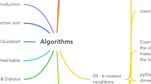
11. 09 - k-nearest neighbors
11.1. feature extraction
11.1.1. what can you use for k-nearest: nem feature extraction, mivel feature extraction kell ahhoz, hogy megold a k-nearest multiple choice: meg lesz adva a feature extraction, ne pipáld be
11.2. Regression
11.2.1. Regression = predicting a response (like a number)
11.2.1.1. You could take the average of their ratings and get 4.2 stars. That’s called regression.
11.2.1.2. Regression is very useful. Suppose you run a small bakery in Berkeley, and you make fresh bread every day. You’re trying to predict how many loaves to make for today.
11.3. classification
11.3.1. Classification = categorization into a group
11.3.2. k = sqrt(n)
11.3.2.1. ha k = 4, mennyi lenne n k = sqrt(n) n = 16
11.4. Cosine similarity doesn’t measure the distance between two vectors. Instead, it compares the angles of the two vectors.
11.5. pythagorean theorem for multiple dimensions - distance between points
11.5.1. euclidean distance
11.5.1.1. a measure of the distance between two points in a multidimensional space.
11.6. optical character recognition
11.7. Naive Bayes classifier.
11.7.1. Spam filters
11.7.2. First, you train your Naive Bayes classifier on some data.
11.8. Predicting the future is hard, and it’s almost impossible when there are so many variables involved.
11.9. OCR = optical character recognition
11.9.1. OCR algorithms measure lines, points, and curves.
11.9.2. The first step of OCR, where you go through images of numbers and extract features, is called training.
11.10. normalization
11.10.1. In the context of k-nearest neighbor (k-NN), normalization refers to the process of scaling the features of the data so that they have a similar range of values. The goal of normalization is to ensure that the features are on a similar scale so that they have equal influence on the k-NN algorithm.
12. 10 - Where to go next
12.1. Bloom filters
12.1.1. probabilistic data structures
12.1.2. False positives are possible.
12.1.2.1. Google might say, “You’ve already crawled this site,” even though you haven’t.
12.1.3. False negatives aren’t possible
12.1.3.1. If the bloom filter says, “You haven’t crawled this site,” then you definitely haven’t crawled this site.
12.1.4. Bloom filters are great because they take up very little space. A hash table would have to store every URL crawled by Google, but a bloom filter doesn’t have to do that.
12.2. HyperLogLog
12.2.1. HyperLogLog approximates the number of unique elements in a set.
12.2.2. Just like bloom filters, it won’t give you an exact answer, but it comes very close and uses only a fraction of the memory a task like this would otherwise take.
12.2.3. count the number of unique x
12.3. Trees
12.3.1. b-tree = special binary tree
12.3.2. red-black tree = self-balanced binary tree
12.3.3. search/insert/delete big O
12.3.4. has to be balanced
12.3.5. Those performance times are also on average and rely on the tree being balanced.
12.4. SHA (secure hash algorithm)
12.4.1. locality insensitive
12.4.2. Simhash
12.4.2.1. locality-sensitive hash function
12.4.2.1.1. If you make a small change to a string, Simhash generates a hash that’s only a little different. This allows you to compare hashes and see how similar two strings are
12.4.3. hash function
12.4.3.1. The hash function for hash tables went from string to array index, whereas SHA goes from string to string.
12.5. Diffie-Hellman algorithm
12.5.1. Diffie-Hellman has two keys: a public key and a private key.
12.6. linear programming
12.6.1. programming technique to optimize, to maximize/minimize
12.6.1.1. simplex algorithm
12.7. Parallel algorithms
12.7.1. The best you can do with a sorting algorithm is roughly O(n log n). It’s well known that you can’t sort an array in O(n) time—unless you use a parallel algorithm! There’s a parallel version of quicksort that will sort an array in O(n) time.
12.7.2. Overhead of managing the parallelism
12.7.3. Load balancing
12.7.4. MapReduce
12.7.4.1. distributed algorithm
12.7.4.1.1. write your algorithm to run across multiple machines. The MapReduce algorithm is a popular distributed algorithm.
12.7.4.2. map function and the reduce function
12.8. inverted index
12.8.1. This is a useful data structure: a hash that maps words to places where they appear. This data structure is called an inverted index, and it’s commonly used to build search engines.
12.9. The Fourier transform
12.9.1. MP3 format
12.9.2. JPG format
12.9.3. great for processing signals.
12.9.4. earthquakes and analyze DNA
12.9.5. Shazam