1. Final steps (optional)
1.1. export it as HTML (keep the **index** file name)
1.2. commit and push
1.3. publish the html
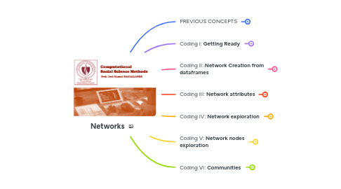
2. PREVIOUS CONCEPTS
2.1. A NETWORK (graph)
2.1.1. nodes
2.1.1.1. attributes
2.1.1.1.1. name?
2.1.1.1.2. age?
2.1.1.1.3. etc
2.1.2. edges or arcs
2.1.2.1. relationship
2.1.2.1.1. undirected or reciprocal
2.1.2.1.2. directed
2.1.2.2. attributes
2.1.2.2.1. weight?
2.1.2.2.2. cost?
2.1.2.2.3. distance?
2.1.3. graph and matrix
2.1.3.1. undirected & unweighted
2.1.3.2. directed and weighted
3. Coding I: **Getting Ready**
3.1. The Libraries needed
3.1.1. verify Rstudio has
3.1.1.1. igraph
3.1.1.2. ggplot2
3.1.1.3. ggraph
3.2. TheData
3.2.1. Create repo for this session
3.2.1.1. Upload file to GitHub
3.2.1.1.1. get URL from GitHub
3.3. The RMD
3.3.1. create a new one for this session
3.3.1.1. save it in the repo for this session
3.3.1.2. name it as **index**
3.4. set the **random seed**
4. Coding II: **Network Creation from dataframes**
4.1. open the file from GitHub
4.2. read the dataframes
4.2.1. R
4.2.1.1. edges represented by pair of nodes
4.2.1.2. adjacency
4.2.1.3. attributes (nodes)
4.3. network from dataframes
4.3.1. create using...
4.3.1.1. edges
4.3.1.1.1. R
4.3.1.2. adjacency
4.3.1.2.1. R
5. Coding III: **Network attributes**
5.1. Adding attributes
5.1.1. R
5.1.1.1. set attribute with a vector
5.1.1.1.1. you have attributes
5.2. using for plotting
5.2.1. R
5.2.1.1. code
5.2.1.1.1. plotting
6. Coding IV: **Network exploration**
6.1. connectedness
6.1.1. A network is “connected” if there exists a *path* between any pair of nodes (undirected networks)
6.1.1.1. R
6.2. density
6.2.1. from 0 to 1, where 1 makes it a ‘complete’ network: there is a link between every pair of nodes.
6.2.1.1. R
6.3. diameter
6.3.1. When two vertices are connected, one can reach the other using multiple egdes. The geodesic is the shorthest path between two connected vertices. Then, the diameter, is the maximum geodesic in a network.
6.3.1.1. R
6.4. assortativity
6.4.1. it is a measure to see if nodes are connecting to other nodes similar to themselves. Closer to 1 means higher assortativity, closer to -1 diassortativity; while 0 is no assortativity.
6.4.1.1. degree
6.4.1.1.1. highly connected nodes tend to contact highly ones(positive). highly connected nodes tend to contact poorly ones (negative)
6.4.1.2. categorical
6.4.1.2.1. nodes in the level of a category tend to contact others in the same level of the same category(positive). nodes in the level of a category tend to contact others in a different level of the same category (negative)
6.4.1.3. numerical
6.4.1.3.1. nodes tend to contact others in the same level of a particular value (positive). nodes with a high value in a particular variable tend to contact others with a low value in that variable (negative)
7. Coding V: **Network nodes exploration**
7.1. The **closeness** of a vertex will tell you how close is a vertex to every other vertex. A vertex with high closeness can share information faster than the rest.
7.1.1. R
7.2. The **eigenvector** of a vertex will tell you how well connected is a vertex; that is, vertices with the highest values are considered the most influential as they are connected to vertices that are also well connected.
7.2.1. R
7.3. The **betweeness** of a vertex will tell you how critical is a vertex to connect vertex that are not connected directly.
7.3.1. R
7.4. exploration
7.4.1. data
7.4.1.1. R
7.4.1.1.1. df
7.4.2. plot
7.4.2.1. all of them
7.4.2.1.1. highlight
8. Coding VI: **Communities**
8.1. Potential communities?
8.1.1. **TRANSITIVITY**: How probable is that two nodes with a common connection, are also connected.
8.1.2. transitivity of **net**/ transitivity of random **net**
8.1.2.1. if higher than one is an evidence!
8.2. Modularity (**Q**)
8.2.1. a standard way to evaluate is communities are well-defined
8.2.1.1. within-community similarity
8.2.1.2. between-community difference
8.3. important algorithm
8.3.1. Girvan-Newman
8.3.1.1. This is a top-down (divisive) method
8.3.1.1.1. repeatedly identifies and removes the "bridge" edge with the highest Edge Betweenness Centrality (the edge that lies on the most shortest paths between communities).
8.3.1.1.2. The best partition is chosen as the one that maximizes Modularity (**Q**) throughout the process.
8.3.2. Louvain
8.3.2.1. This is a bottom-up (agglomerative) method
8.3.2.1.1. It starts with every node as its own community and iteratively merges and moves nodes between communities until no further move can increase the Modularity score.
