

1. Coding I: **Getting Ready**
1.1. The Libraries needed
1.1.1. verify Colab has
1.1.1.1. pysal
1.1.1.1.1. libpysal
1.1.1.1.2. esda
1.1.1.2. pandas
1.1.1.3. geopandas
1.2. using GeoPandas
1.2.1. activate
1.2.2. use **read_file** function
1.2.2.1. What will you get?
1.2.2.1.1. Data Frame
1.2.2.1.2. Geo Data Frame
1.2.3. using geopandas:
1.2.3.1. check CRS
1.2.3.1.1. check if projected
1.2.3.2. check geom types
1.2.3.3. check usual DF features
1.2.3.3.1. (data) column types
1.2.3.3.2. shape (count of rows/columns)
1.2.3.3.3. head/tail
1.2.3.3.4. use a column as **row index**?
1.2.3.4. subsetting maps
1.2.3.4.1. USA
1.2.3.4.2. PERU
2. Coding II: **Neighborhood**
2.1. previous steps
2.1.1. activate PYSAL!
2.1.1.1. from libpysal.graph import Graph
2.1.1.1.1. terminology
2.1.2. set random seed
2.1.2.1. so you can get my results
2.2. geometries touch each other in any portion of their boundaries?
2.2.1. YES: contiguity
2.2.1.1. rook
2.2.1.1.1. you are my neighbor if we share at least a line segment on our boundaries
2.2.1.2. queen
2.2.1.2.1. you are my neighbor if we share at least a boundary point
2.2.1.3. either may generate isolates
2.2.1.4. Notice we created these wide matrices for pedagogical purposes. It is a bad idea if you have many columns and rows.
2.2.2. NO
2.2.2.1. Close **enough** to be considered a neighbor
2.2.2.1.1. YES: proximity
2.2.2.1.2. NO: not a neighbor (am I an ISLAND?)
2.2.2.2. requires point coordinates to compute distance
3. Coding III
3.1. **Normalization**
3.1.1. all previous matrices SUM by ROW
3.1.1.1. the sum by row
3.1.1.1.1. unnormalized weights
3.1.2. normalized weights
3.1.2.1. transforming values per row
3.1.2.1.1. a row adds to 1 (ONE)
3.2. **The spatial lag**
3.2.1. **How are each of us doing...?** (related to a social variable)
3.2.1.1. choropleth: **share of population that completed high school **
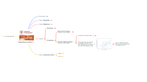
3.2.2. **How is the neighborhood doing ...?** (related to a social variable)
3.2.2.1. Compute the normalized matrix
3.2.2.1.1. to weight social data values of neighbors
3.2.2.2. Each polygon lag is the average of the neighbor values (the social data) weighted by the normalized row values of the adjacency matrix.
3.2.2.2.1. here, my education level (X) follows a direct relationship with my neighbors level (Y)
4. Coding IV: **Spatial Autocorrelation**
4.1. Global
4.1.1. my variable values is affected by my neighbors' variable values?
4.1.1.1. Moran's I
4.1.1.1.1. coefficient (similar to Pearson's R) measuring the relationship between a variable and its lag
4.2. Local
4.2.1. my local situation is affected by my neighbors situation?
4.2.1.1. Moran's LISA
4.2.1.1.1. reveals autocorrelation clusters