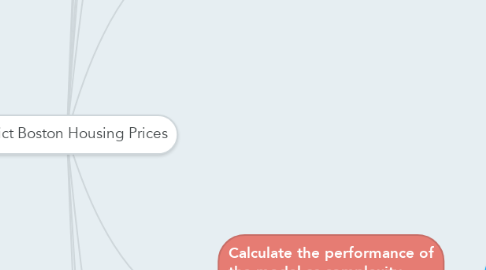
1. Load the Boston Dataset
1.1. def load_data():
1.1.1. boston = datasets.load_boston()
1.1.1.1. return boston
2. Calculate the Boston housing statistics
2.1. def explore_city_data(city_data):
2.1.1. housing_prices = city_data.target
2.1.2. housing_features = city_data.data
2.2. Number of Houses?
2.3. Number of features?
2.4. Minimum Price?
2.4.1. np.min(housing_prices)
2.5. Maximum Price?
2.5.1. np.max(housing_prices)
2.6. Calculate mean Price?
2.6.1. np.mean(housing_prices)
2.7. Calculate median Price?
2.7.1. np.median(housing_prices)
2.8. Calculate standard deviation?
2.8.1. np.std(housing_prices)
3. Calculate and return the appropriate error performance metric
3.1. def performance_metric(label, prediction):
3.1.1. error = metrics.mean_squared_error(label, prediction)
3.1.2. return error
4. Randomly shuffle the sample set. Divide it into 70 % training and 30% testing data
4.1. def split_data(city_data)
4.1.1. Get the features and labels from the Boston housing data
4.1.1.1. X, y = city_data.data, city_data.target
4.1.1.2. X_train, X_test, y_train, y_test = cross_validation.train_test_split(X, y, random_state=0)
4.1.1.3. return X_train, y_train, X_test, y_test
5. Calculate the performance of the model after a set of training data.
5.1. def learning_curve(depth, X_train, y_train, X_test, y_test):
5.1.1. Vary the training set size so that we have 50
5.1.1.1. sizes = np.linspace(1, len(X_train), 50
5.1.1.2. train_err = np.zeros(len(sizes))
5.1.1.3. test_err = np.zeros(len(sizes))
5.1.1.4. print "Decision Tree with Max Depth: "
5.1.1.5. print depth
5.1.1.6. for i, s in enumerate(sizes):
5.1.1.6.1. Create and fit the decision tree regressor model
5.1.1.6.2. Find the performance on the training and testing set
5.1.1.6.3. Plot learning curve graph
6. Plot training and test error as a function of the training size
6.1. def learning_curve_graph(sizes, train_err, test_err):
6.1.1. pl.figure()
6.1.2. pl.title('Decision Trees: Performance vs Training size')
6.1.3. pl.plot(sizes, test_err, lw=2, label='test error')
6.1.4. pl.plot(sizes, train_err, lw=2, label = 'training error')
6.1.5. pl.legend()
6.1.6. pl.xlabel('Training Size')
6.1.7. pl.ylabel('Error')
6.1.8. pl.show()
7. Calculate the performance of the model as complexity increases
7.1. def model_complexity(X_train, y_train, X_test, y_test):
7.1.1. print "Model Complexity: "
7.1.2. We will vary the depth of decision trees from 2 to 25
7.1.2.1. max_depth = np.arrange(1, 25)
7.1.2.2. train_err = np.zeros(len(max_depth))
7.1.2.3. test_err = np.zeros(len(max_depth))
7.1.3. Setup a decision tree regressor so that it learns a tree with depth d
7.1.3.1. for i, d in enumerate(max_depth):
7.1.3.2. regressor = DecisionTreeRegresor(max_depth=d)
7.1.4. Fit the learner to the training data
7.1.4.1. regressor.fit(X_train, y_train)
7.1.5. Find the performance on the training set
7.1.5.1. train_err[i] = performance_metric(y_train, regressor.predict(X_train))
7.1.6. Find the performance on the testing set
7.1.6.1. test_err[i] = performance_metric(y_test, regressor.predict(X_test))
7.1.7. plot the model complexity graph
7.1.7.1. model_complexity_graph(max_depth, train_err, test_err
8. Plot training and test error as a function of the depth of the decision tree learn.
8.1. def model_complexity_graph(max_depth, train_err, test_err):
8.1.1. pl.figure()
8.1.2. pl.title("Decision Trees: Performance vs Max Depth")
8.1.3. pl.plot(max_depth, test_err, lw=2, label = 'test error'
8.1.4. pl.plot(max_depth, train_err, lw=2, label = 'training error')
8.1.5. pl.legend()
8.1.6. pl.xlabel('Max Depth')
8.1.7. pl.ylabel('Error')
8.1.8. pl.show()
9. Find and tune the optimal model. Make a prediction on housing data.
9.1. def fit_predict_model(city_data):
9.1.1. Get the features and labels from the Boston housing data
9.1.1.1. X, y = city_data.data, city_data.target
9.1.2. Setup a Decision Tree Regressor
9.1.2.1. regressor = DecisionTreeRegressor()
9.1.2.2. parameters = {'max_depth':(1,2,3,4,5,6,7,8,9,10)}
9.1.3. 1. Find the best performance metric
9.1.3.1. scorer = metrics.make_scorer(performance_metric, greater_is_better = False)
9.1.4. 2. Use gridsearch to fine tune the Decision tree regressor and find the best model
9.1.4.1. reg = grid_search.GridSearchCV(regressor, parameters, scoring=scorer, verbose=True)
9.1.5. Fit the learner to the training data
9.1.5.1. print "Final Model:"
9.1.5.2. print reg.fit(X, y)
9.1.6. Use the model to predict the output of a particular sample
9.1.6.1. x = [11.95, 0.00, 18.100, 0, 0.6590, 5.6090, 90.00, 1.385, 24, 680.0, 20.20, 332.09, 12.13]
9.1.6.2. y = reg.predict(x)
9.1.6.3. print "House: " + str(x)
9.1.6.4. print "Prediction: " + str(y)
10. Analyze the Boston housing data. Evaluate and validate the performance of a Decision Tree regressor on the housing data. Fine tune the model to make prediction on unseen data.
10.1. def main():
10.1.1. Load data
10.1.1.1. city_data = load_data()
10.1.2. Explore the data
10.1.2.1. explore_city_data(city_data)
10.1.3. Training/test dataset split
10.1.3.1. X_train, y_train, X_test, y_test = split_data(city_data)
10.1.4. Learning Curve Graphs
10.1.4.1. max_depths = [1, 2, 3, 4, 5, 6, 7, 8, 9, 10]
10.1.4.2. for max_depth in max_depths:
10.1.4.2.1. learning_curve(max_depth, X_train, y_train, X_test, y_test)
10.1.5. Model Complexity Graph
10.1.5.1. model_complexity(X_train, y_train, X_test, y_test)
10.1.6. Tune and predict model
10.1.6.1. fit_predict_model(city_data)

