Hourly Runoff Forecast at Different Leadtime for a Small Watershed using Artificial Neural Networks

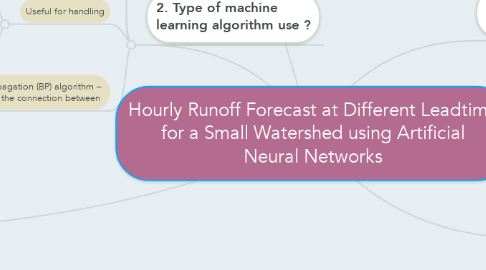
1. 3. Specific method/algorithm to solve the problem (methodology) ?

1.1. Multilayer Perceptron Neural Network (MLP)

1.1.1. Two-layer feedforward network

1.1.2. The transfer function used

1.1.2.1. Hidden layer --> tansigmoid (tansig)

1.1.2.2. Output layer --> linear transfer (purelin)

1.1.3. Number of hidden neurons determined through training

1.1.3.1. Scaled Conjugate Gradient (TRAINSCG).

1.1.3.2. Variable Learning Rate Backpropagation (TRAINGDX)

1.1.3.3. Powell-Beale Restarts (TRAINCGB)

1.1.4. Flow of MLP

1.1.4.1. Input layer to---> Hidden layer (tansig function)

1.1.4.2. Hidden layer to---> Output layer (purelin function)

1.2. Recurrent (REC) Network (known as Elman Network)

1.2.1. Two layer feedback network

1.2.2. Allows Elman networks to :

1.2.2.1. Learn to recognize

1.2.2.2. Generate temporal patterns & spatial patterns

1.2.2.3. Stores values from the previous time step

1.2.2.4. Use them in the current time step.

1.2.3. Number of hidden neurons determined through training

1.2.3.1. Scaled Conjugate Gradient (TRAINSCG).

1.2.3.2. Variable Learning Rate Backpropagation (TRAINGDX)

1.2.3.3. Powell-Beale Restarts (TRAINCGB)

1.2.4. Useful in areas such prediction where time plays an important role.

1.2.4.1. MUST have enough hidden neurons to divide the input space in a useful way

1.2.4.2. Perform better when there are more hidden neurons than actually required.

1.2.4.3. When fewer neurons, Elman network is less able to find the most appropriate weights for hidden neurons since the error gradient is approximated

2. 2. Type of machine learning algorithm use ?

2.1. Supervised Learning Of Neural Networks

2.2. Called Backpropagation Neural Network (BPNN)

2.3. Useful for handling

2.3.1. Large volume of real-time

2.3.2. Non-stationary natural phenomena

2.3.3. Non-linear natural phenomena

2.4. Backpropagation (BP) algorithm – Discover the connection between

2.4.1. The domain concepts contained in the learning object

2.4.2. The learner’s learning need

3. 1. Paper/manuscript is all about ?

3.1. Real-time flood forecasting models using artificial neural networks (ANNs)

3.1.1. input of rainfall and runoff data only.

3.2. ANNs were trained and tested in order to select the best performance ANNs.

3.2.1. Different training algorithm

3.2.2. Different number of hidden neurons

3.2.3. Different learning rate

3.2.4. Different number of antecedent hours

3.3. Optimal configuration of ANNs model obtained

3.3.1. Will be adopted to forecast the runoff at 3, 6, 12 and 18 hours ahead for Bedup basin.

3.4. Two types of neural networks

3.4.1. Multilayer Perceptron (MLP) network

3.4.2. Recurrent (REC) network.

4. 5. Type of machine learning algorithm use ?

4.1. Rainfall-runoff relationships are among the most complex hydrologic phenomena

4.1.1. The conceptual models developed by Hydrologists for simulating runoff composed of a large number of parameters and the interactions are highly complicated

4.1.2. The accuracy of conceptual model simulation is very subjective and highly depends on the modeler’s ability and understanding of the model

4.1.3. Therefore, ANNs is applied to model rainfall-runoff.

5. 4. The machine learning algorithm implemented? (methodology)

5.1. MLP and REC networks - applied to train and test the hourly rainfall-runoff model

5.2. The performance of MLP and REC are evaluated from FOUR MAIN perspectives including:

5.2.1. Different types of training algorithms

5.2.2. Different number of antecedent hours

5.2.3. Different number of hidden neurons

5.2.4. Different learning rate values

5.3. Investigating the effect of the number of antecedent hours on the performance of MLP and REC. The input data for this :

5.3.1. Antecedent hour precipitation

5.3.2. Antecedent hour discharges

5.3.3. The rainfall of the current hour

5.4. The output for all this 3 input is hourly runoff

5.4.1. A single objective function named as Mean Squared Error (MSE) is used to calibrate the model.

5.4.2. The accuracy of the simulation results are measured with coefficient of correlation (R) and Nash-Sutcliffe coefficient (E2).

5.4.3. The closer R and E2 values to 1.0 indicate better results obtained.